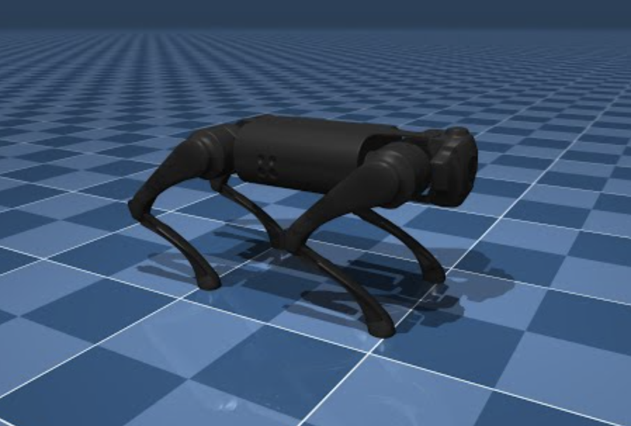
Reinforcement learning (RL) is like teaching your dog new tricks, but instead of treats, we use rewards and penalties. In this guide, we’ll dive into training a reinforcement learning agent for a Unitree Go1 quadruped robot using the MuJoCo physics engine for simulation and MATLAB’s Reinforcement Learning Toolbox for training. Buckle up, it’s going to be a fun ride!
Prerequisites
Before we jump in, make sure you have the following:
Python and dependencies: Create a Python virtual environment for your project.
python -m venv env
source ./env/bin/activate
Install the Gymnasium and MuJoCo libraries.
pip install gymnasium[mujoco]
The Go1 robot model is found in the MuJoCo Menagerie repository. Add the repository as a submodule.
git submodule add https://github.com/google-deepmind/mujoco_menagerie.git
MATLAB and Reinforcement Learning Toolbox: Follow the instructions on the MathWorks website to install MATLAB and the Reinforcement Learning Toolbox.
Creating the Simulation Model
MuJoCo’s simulation for the Unitree Go1 robot handles complex interactions between the robot’s limbs and the environment, ensuring realistic simulation of forces, torques, and contacts. MuJoCo also integrates seamlessly with Gymnasium, a toolkit for developing and comparing RL algorithms. By tweaking the Mujoco/Ant-v5 framework, we can make it behave like our Unitree robot. This involves adjusting the XML model file, reward weights, control costs, and other environment specifications. Gymnasium actually has a good article on this. See it here.
Create a Python file go1.py in your project folder.
import gymnasium
from robot_descriptions import go1_mj_description

def create_env():
  return gymnasium.make(
    'Ant-v5',
    xml_file=go1_mj_description.MJCF_PATH,
    forward_reward_weight=1,
    ctrl_cost_weight=0.05,
    contact_cost_weight=5e-4,
    healthy_reward=1,
    main_body=1,
    healthy_z_range=(0.195, 0.75),
    include_cfrc_ext_in_observation=True,
    exclude_current_positions_from_observation=False,
    reset_noise_scale=0.1,
    frame_skip=25,
    max_episode_steps=1000,
  )
The environment has the following specifications.
Observation Space:
- Positions and velocities of the robot’s joints, body position, center of mass position and velocity, and contact forces on the robot’s limbs.
- Represented as a continuous vector of
115real numbers.
Action Space:
- 12 torque values applied to the robot’s joints.
- Bounded by the maximum and minimum torque values the robot’s actuators can produce.
Reward Function:
- Encourages forward movement while penalizing inefficient or unsafe behaviors.
- Forward Reward: Proportional to the forward velocity.
- Control Cost: Penalizes large torques.
- Contact Cost: Penalizes excessive contact forces.
- Healthy Reward: Constant reward for staying upright.
Termination Logic:
- Episode ends if the robot’s body falls below or exceeds a certain height.
To integrate this environment in MATLAB, we will call Python from MATLAB using the pyrun function.
result = pyrun("some_python_function()", "result");
You can also pass MATLAB variables to Python functions:
inputVar = 10;
result = pyrun("some_python_function(inputVar)", "result", inputVar=inputVar);
Open MATLAB and run the following code to create the environment in MATLAB:
pyrun("import go1");
penv = pyrun("env = go1.create_env()","env")
And that’s it! The penv variable now stores information about the Go1 robot in MATLAB.
Tip: Opening MATLAB from a terminal with the activated virtual environment automatically configures the dependencies within the MATLAB process. On macOS you can use this command /Applications/MATLAB_R2024b.app/bin/matlab, after changing it to the correct MATLAB version on your computer.
Creating a MATLAB Reinforcement Learning Environment
MATLAB’s environments infrastructure can be used to generate data for training agents. We’ll wrap the Gymnasium environment within a MATLAB environment.
First, define the observation and action specifications:
numObs = double(penv.observation_space.shape{1});
numAct = double(penv.action_space.shape{1});
action_low = double(penv.action_space.low);
action_high = double(penv.action_space.high);
Create the specifications:
obsInfo = rlNumericSpec([numObs,1]);
actInfo = rlNumericSpec([numAct,1]);
actInfo.LowerLimit = action_low;
actInfo.UpperLimit = action_high;
Define a function stepFun.m for the environment:
function [nextobs,reward,isdone,info] = stepFun(penv,action,info)
   pyAction = py.numpy.array(action);
   pyStepOut = penv.step(pyAction);
   nextobs = double(pyStepOut{1});
   reward = double(pyStepOut{2});
   isdone = pyStepOut{3} || pyStepOut{4};
end
Create a reset function resetFun.m:
function [obs,info] = resetFun(penv)
   pyResetOut = penv.reset();
   obs = double(pyResetOut{1});
   info = [];
end
Finally, create the environment object:
step = @(action,info) stepFun(penv,action,info);
reset = @() resetFun(penv);
env = rlFunctionEnv(obsInfo,actInfo,step,reset);
Designing a Soft Actor-Critic (SAC) Agent
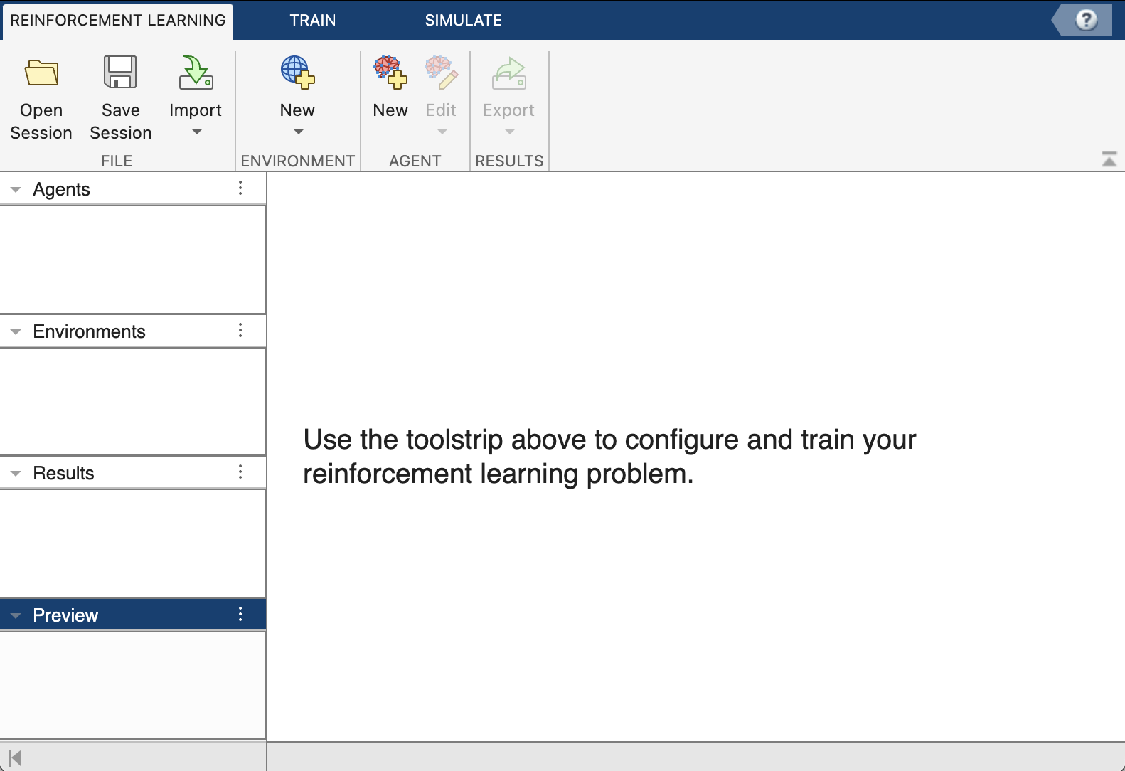
The Reinforcement Learning Designer app in MATLAB is a powerful tool that simplifies the process of developing reinforcement learning agents. It offers an interactive graphical interface where users can design, train, and simulate RL agents without the need for extensive coding. The app allows you to import custom environments and configure agent algorithms. Additionally, it provides visualization tools to analyze the performance of the agents during training and simulation. This makes it an invaluable resource for both beginners and experienced practitioners in the field of reinforcement learning.
Open the app in the MATLAB session:
reinforcementLearningDesigner
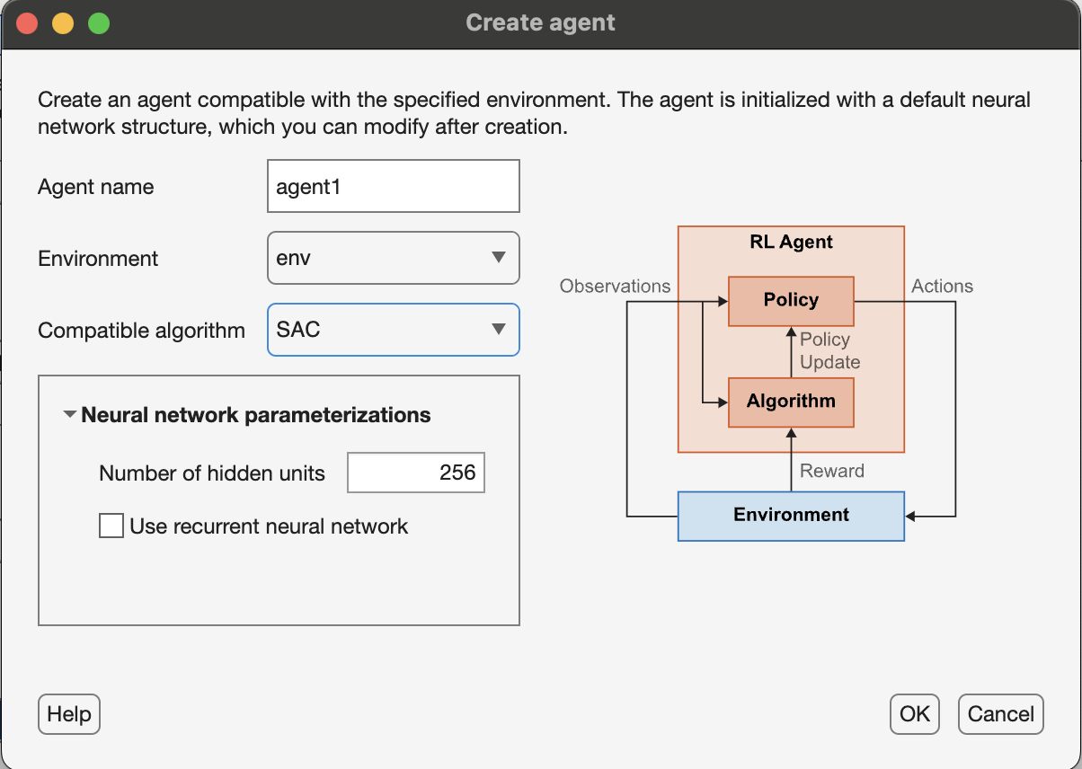
Import the environment in the app workspace. Click Import and choose the env object.
Create an agent by clicking the New button under the Agent section. Select the SAC algorithm and a choice of hidden units (256), and click Ok.
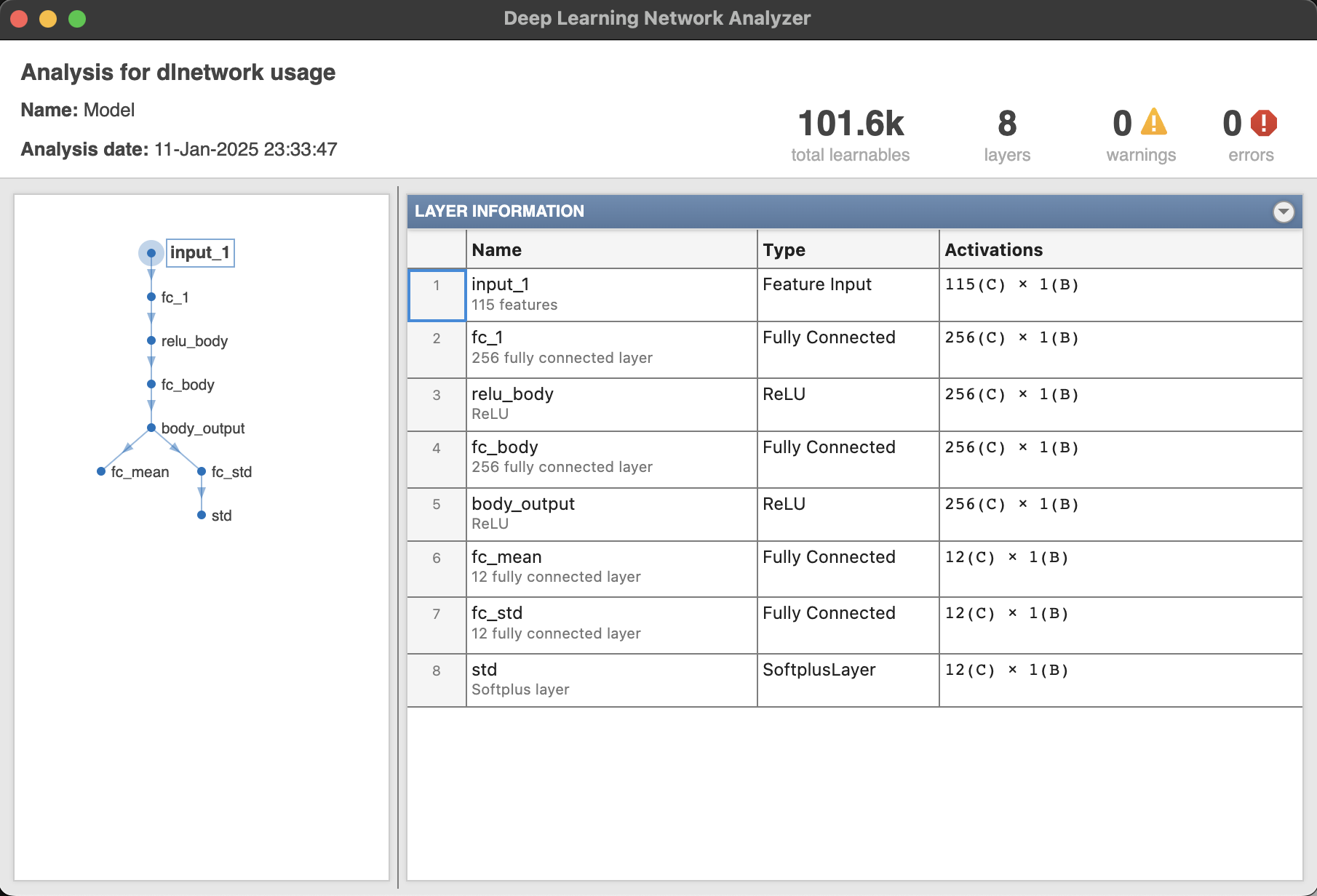
Analyze the actor and critic networks using the View Actor/Critic Model button. The following image shows the actor network responsible for computing actions. Typically, the network maps states to a probability distribution over actions. In the context of the SAC algorithm, the actor network outputs parameters of a stochastic policy, often modeled as a Gaussian distribution. This allows the agent to explore the action space effectively. The network usually consists of multiple layers, including input, hidden, and output layers, with the hidden layers employing activation functions like ReLU to introduce non-linearity and enable the network to learn complex state-action mappings.
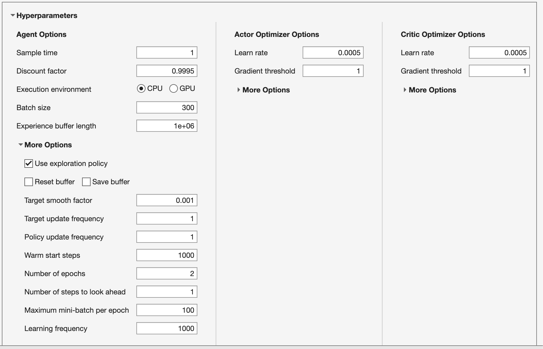
Although the agent comes preconfigured with a default set of hyperparameters it may not be sufficient for this problem. Hyperparameter tuning can be challenging due to the complex interactions between parameters; a simplistic approach involves keeping the learning rates low, using gradient thresholding, employing a large batch size to stabilize gradients, and adjusting the learning frequency to allow for sufficient data collection between learning steps.
Tune the hyperparameters:
- Actor and critic learning rates
5e-4with gradient threshold1. - Batch size
300. - Discount factor
0.995. - Experience buffer length of
1e6.
Under More Options:
- Learning frequency
1000. - Number of epochs
2. - Warm start steps
1000.
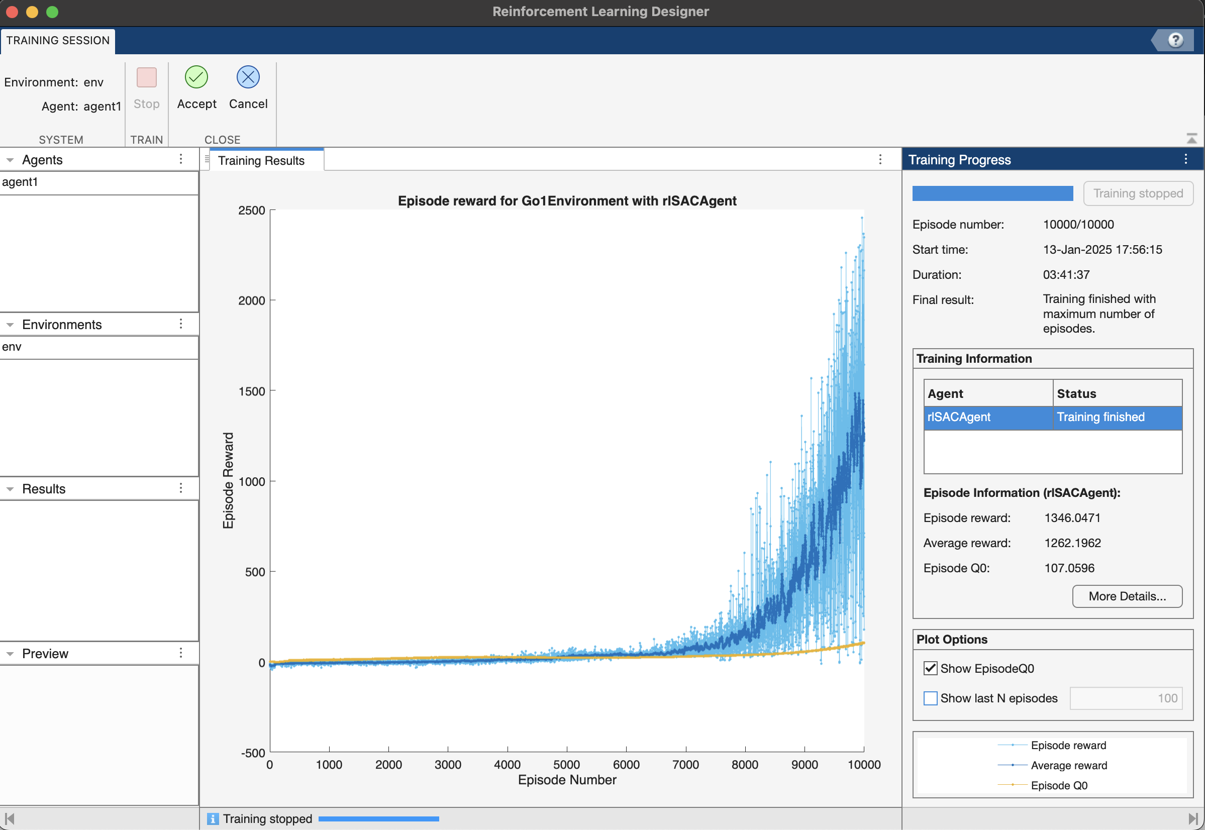
Training the RL Agent
With the simulation model and RL agent in place, we can start the training process. This involves running multiple episodes of the simulation, where the agent interacts with the environment and learns from the rewards it receives.
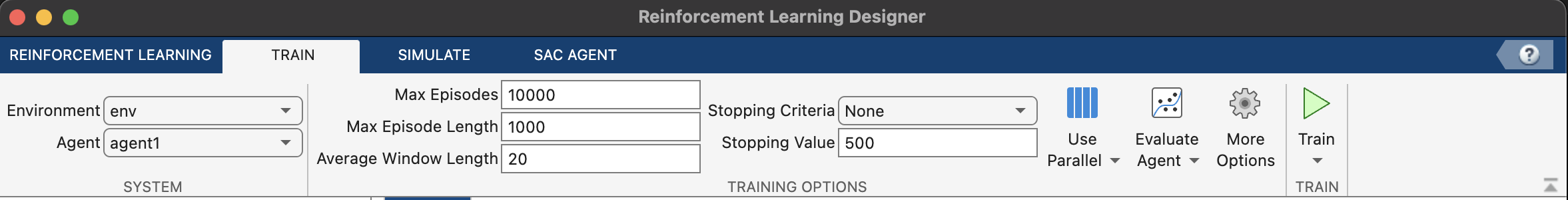
Navigate to the Train tab, and set the following training options:
- Max episodes
10000. - Max steps per episode
1000. - Averaging window length
20. - Stop training criteria
none.
Click the Train button to start training. Once the training is finished, Accept the training results in the app workspace.
Tip: Save the app session after training to save progress. You can also reload the app session for later use.
Evaluating the Trained Agent
After training, we will evaluate the performance of the RL agent by running it in simulation and observing its behavior.
Navigate to the Simulate tab and adjust the parameters:
- Number of episodes
5. - Max episode length
1000.
Click Simulate to run simulations.
Here is a video recording of the trained agent.
As you can see, the robot makes a valiant effort to move forward, though its gait could use some refinement. More training will be needed to perfect its movements, but that’s a challenge for another day. In this guide, we’ve laid the groundwork for seamlessly connecting Python-based environments with MATLAB, setting the stage for more advanced robotics adventures. Happy coding!
Info: The environment described here does not automatically record videos. Use the scripts in the GitHub repository to create a RecordVideo wrapper around the environment. You may need to download and install ffmpeg software for recording.
Conclusion and Future Work
Interested to use this work? Fork my repository here.
That’s it for this one. Stay tuned for more exciting robotics topics! Whether you’re a beginner or an experienced practitioner, there’s always something new to learn and discover. Keep experimenting, keep coding, and stay curious!